Bibliography

Glassner, A. S. (1990). An introduction to ray tracing. San Diego, Ca: Academic Press.

Phong Reflection Model (2011, July 10). General format. Retrieved from

http://en.wikipedia.org/wiki/Phong_reflection_model

Sunday, D. (2011, August 5). Intersections of Rays, Segments, Planes and Triangles in 3D Retrieved from

http://softsurfer.com/Archive/algorithm_0105/algorithm_0105.htm

Parting Words

Building a ray tracer has been the enlightening experience it was supposed to be; Even on such a small scale, it has revealed to the author a Pandora's box of avenues to explore, confident that a solid foundation has been established first. Even the implementation itself was educational as every addition to the program necessitated some form of refactoring, to be in tune with proper OOP techniques. 


Elegant programming is a challenge in itself: A performing application will remain a task that requires careful planning. The author will remind the reader that little attention has been given to improving the overall performance of the software,  as the main focus was to achieve results. The performance issue remains secondary at the moment, but will be addressed as more complex application will eventually necessitate such improvements to remain practical.  


Apart from the implementation, the other challenges of applying linear algebra concepts were also enlightening, and clearly worth pursuing as a topic in itself.


The realm of image rendering being virtually limitless, some avenues the author would like to pursue became obvious as he progressed: Refraction, texture mapping, polygon mesh development, will surely be addressed in the near future.

Ray Polygon Intersection

The next element we will try to render could be considered one of the most important building blocks in ray tracing imagery: The polygon. Again, in our quest for simplicity and efficiency we will focus our efforts on the smallest possible polygon, a triangle.

A three-sided polygon: Some characteristics
The triangle polygon possesses numerous characteristics that make it the perfect building block for more complex structures to be rendered. 


Each triangle is inscribed in its own plane
The first and most important characteristic would be that the triangle is the only polygon that is inscribed in a plane. The three vertices that compose the triangle will occupy a common plane, no matter their distance or relative position. The assurance that a polygon is flat is a critical aspect of its usefulness. By finding the cross product of vectors implied by the polygons's vertices, we can find the normal to the polygon's plane. Once this normal becomes available, we can then apply any desired shading technique on the polygon's surface.


Polygons can share vertices and edges
Another advantage of polygons, not just triangles in this case, is that they can have common vertices or edges. This characteristic is used in one of the oldest 3 D modelling data structure, the polygon mesh. Since each polygon can possibly have edges of different lengths, this flexibility can allow for the creation of smooth appearing larger volumes. The illusion of smoothness in the curves of the object can be controlled by either augmenting the number of polygons involved in the mesh, or by other more computationally economical rendering techniques like normal manipulation or texture mapping, topics that, due to time limitations, will not be addressed in great detail in the present blog.

Dolphin triangle polygon mesh.
(Image courtesy of Wikipedia)

As the complexities inherent to creating polygon mesh are beyond the scope of this blog, we will now examine the ray polygon intersection:

First step in Ray Polygon intersection: Ray plane intersection

Glassner[1] suggests a three step approach into dealing with ray-polygon intersection:

1. Find the plane the polygon is inscribed in
2. Verify if the ray intersects with the plane
3. If the intersection is positive, verify that the ray is within the polygon

Finding the polygon's plane

There are many way to find a specific plane that is related to a series of vertices: The method we chose involves creating two vectors from two pairs of points from our polygon, as those vertices are instantiated when the polygon object is created. We then find the normal of these vectors through the vector cross product operation.


Linear algebra concept: Cross Product
The cross product of 2 vectors will create a third vector perpendicular to both original vectors simultaneously. This cross product can be determined by the vertice's coordinates.


Cross product utility method
Since the cross product is a relatively simple formula, a java utility method can easily be implemented. It is a member method of the polygon class and is called every time a polygon object is created.

public double[] get_normal(){

// we will find vector u and v and then find n with cross product

// create vectors u and v from vertices of triangle, save them in object members

for(int i = 0 ; i < 3 ;i++){

    this.u[i] = vertice1[i] - vertice0[i];

    this.v[i] = vertice2[i] - vertice0[i];

}

this.n[0] = (u[1] * v[2]) - (u[2] * v[1]);// x coordinate of normal

this.n[1] = (u[2] * v[0]) - (u[0] * v[2]);// y coordinate of normal

this.n[2] = (u[0] * v[1]) - (u[1] * v[0]);// z coordinate of normal

for(int i = 0 ; i < 3 ; i++)

    if(this.n[i] == -0.0)

      this.n[i] = 0.0;

// normalise n before sending it

this.n = this.normalise_vector(this.n);

// we can now find ABCD of plane to save them for later use for D, just use abc on one point from triangle

this.plane[0] = this.n[0]; //A

this.plane[1] = this.n[1]; //B

this.plane[2] = this.n[2]; //C

this.plane[3] = -1 * (this.n[0] * vertice0[0] + this.n[1] * vertice0[1]+ this.n[2] * vertice0[2]); //D

return n;

}

Defining the plane: Cross Product and a point
The implicit polygon's plane equation can then be derived from the polygon's normal and by choosing one vertice.  Once again, the ray plane intersection can be expressed in terms of t distance units by substituting the ray equation into the plane's equation and solving for t. The complete details of those operations can be found in Glassner[1] (pp 50-51).
Finding if the ray intersects with the inside of the polygon
The author will mention that of all the algorithms used up to now, the one used to verify if the ray strikes the polygon on the inside is the most complicated. After evaluation, the author has chosen to steer away from Glassner's solution of firing in-plane rays from the ray plane intersection point [1] (pp 53 54) to a solution involving parametric equations, cross and dot products derived from those already acquired. The complete solution can be found here Ray polygon intersection 
The author will readily admit that some elements of this solution involves linear algebra concepts that have not yet been fully understood, which made the implementation somehow time consuming, but still successful.

Success! Our first Phong shaded polygon

Polygons and the Phong Reflection Model
One of the aspects of the polygon shading algorithm that remains clearly understood is the Phong model can readily be applied to polygons once their normal have been found. One important characteristic of in-plane polygons is the polygon's normal remains constant on all the points of the surface of the polygon. Since the angle of the ray with the normal will change depending on which pixel is rendered, the Phong model will add nuances to the colours of the object, creating the illusion of three dimensions. In the other example below, a horizontal polygon is stretched to a large size to simulate a flat surface extending to the horizon.

Polygon stretched to simulate a horizontal plane

Creating more complex shapes out of polygons: A complex task

Once the rendering of simple polygons has been achieved, it will be easy to notice the inherent complexity in creating larger shapes; Polygons, opposed to spheres, have no definite  shape. This will create problems when wanting to build more complex elements as finding the  appropriate vertice coordinates cannot easily be guessed. Even building a simple cube will require 12 polygons. If this cube is to be shifted as so to be visible in a perspective point of view, finding the vertice's coordinates will be daunting. The solution to this problem resides in the use of transformation formulas which will recompute the coordinates according to the nature of the transformations, be it rotation, shearing, stretching, etc...  This topic will be investigated by the author in the future.

Reflections

As the foundations of the ray tracer application have now been laid down, the next implementation stage can be set; Reflections.


The relationship of light with objects could be reduced to 2 interactions; Either light bounces off an object, either partially or completely, or it traverses the object. Traversing the object, an effect known as refraction, shares some characteristics with reflections: Both reflection and refraction mechanisms possess incident and reflected rays, although the similarities end there. The main difference between the two effects would be that in reflection, the ray remains on the same side of the normal of the surface involved, while in refraction, the ray goes into the opposite side of the normal involved. This is illustrated below.

Image from omniadiamonds.com

We will now focus our attention on ray tracer reflection issues. Refraction being a complete topic in itself, it will be left out for future explorations. 


Reflections applied to ray tracing
It is fortunate that the tools we have already developed for rendering can be applied to simulate object reflections. They simply need to be adapted to fill that purpose. The key element in reflection would be that instead of having a ray of light coming from a light source, bouncing on an object into our eye,  (we here remind the reader that we are describing forward ray tracing for clarity) we have the ray bounce on a first object onto a second one, and then having this second bounce go into our eye. 


Intensity of the reflected light 
Now that we have established the basic elements for reflection to occur, i.e. two objects at the least, positioned in such a way that the light reflecting off one object is directed at the other, we must focus our attention on how to establish the final light intensity that would enter our eye. 
The solution lies in adding all the light intensities involved at every step of the reflection; In the simplest of scenarios, we compute the light intensity of the first object at the point of contact, then this intensity is added to that of the other object, and this sum of intensities for this particular ray are then sent to the eye.
How do we calculate the intensities to be sent to other object?  The solution lies in using the Phong model at each point involved in the reflection process; as shown in the illustration below.

The reflection process

To find the final light intensity at point VP' we must substitute VP' for VP in the Phong model. By having VP' as new viewpoint, we can then calculate the intensity of sphere A at its point of reflection. The next step would be to calculate the intensity at VP' without the reflection added.  This is simply achieved by applying the Phong model in the manner now familiar to us.
Here is a typical reflection example created with the application:

Two spheres reflecting in each other.

Recursive possibilities 
It is interesting to note that a reflection algorithm could be implemented in a recursive fashion, enabling the superimposition of multiple reflections, creating the double mirror effect. The Simple Ray Tracer application, due to the inherent complexity of establishing a proper recursive reflection method, has instead implemented a non-recursive reflection method that can only create single level reflections in objects. Perhaps, in future developments, such a recursive method will be used.


The reflection coefficient: How much light to reflect?
Another interesting aspect of reflection lies in evaluating how much light an object actually reflects in opposition to how much it absorbs. If an object reflects 100% of the light it receives, we could say that the object does not have a colour of its own, but is only visible by the reflections it creates. 
An object could also be totally non reflexive and therefore be invisible; But reality imposes the idea that all objects have different reflexive properties. We can quantify this in our program by 
adding another data member to our objects a reflection index.  The reflection index is a value of range 0.0 to 1.0 that basically subtracts a portion of the light intensity of an object to replace that portion with the intensity of the reflection. A reflection index of 0.3 for instance would remove 0.3 * the intensity of the object and replace it the intensity of the reflection. A reflection index of 1.0 replaces the intensity of the object entirely by the reflection. The underlying colour disappears. At this point in the implementation, the reflection index serves only a Boolean value. Each object is either entirely or totally non reflexive, a non-reflexive object still being visible as the index only affects the points of the object where reflections occur.

Rendered scene with no reflection

The same scene, with reflection added.

Antialiasing

Aliasing: Unwanted Image artifacts
An interesting aspect of image rendering lies in the elimination or, if not possible, of the attenuation of image artifacts; i.e. visible defects in the image. These defects can range from unrealistic lighting effects to awkward looking reflections. But in a digital pixel-based image, none is more obvious than what is referred to as aliasing. Aliasing, refers to the problem that a digital image being built out of discrete elements, here pixels, will have certain of those elements which should have been distinct, copy each other. For the pixels in an image, this aliasing artifact is referred to as "jaggies". The jaggies are mostly found in areas where there is a sudden change in light intensity or colour,  creating instead of a smooth line, a "jagged" edge.


Antialiasing
Antialiasing, as its name suggest, is the set of methods used to remove or reduce pixel related artifacts. There are many algorithms that can be used to alleviate this problem: Supersampling and Stochastic (or random) ray sampling are described in Glassner's[1].


Supersampling
The method we have chosen to experiment with will be supersampling. It is the simplest, and the most adaptable to our present implementation. The concept is very simple: Instead of having one ray per pixel which could create a hard border between the edge of a sphere and its background, we fire multiple rays within the viewing window's pixel area. We then average out the intensities for the particular pixel and send that average intensity to the image buffer. The result is a much smoother image, 


The ViewPoint class possesses a member method antialiasing_vectors that adds into the pixel area of the viewing window 4 evenly distributed coordinates where a ray will be sent to. This is easily done by changing the area's offsets.

Supersampling vs single ray sampling

Adding more rays will obviously augment rendering time; But since performance is not the issue, the results are worth the wait. We can easily compare an antialiased image to its non-antialiased version, by inserting the 'a' command line argument when launching the ray tracer application. Here are comparison results:

Rendered image with antialiasing at OFF

Same image with antialiasing

The antialiasing is best seen here with close-ups of the previous images:

Antialising is OFF

Antialiasing is ON

There are more efficient ways of reducing the aliasing effects than just by augmenting the number of rays per pixel area. Stochastic antialiasing applies a random spreading of the rays inside the pixel area, which will have similar effects as supersampling, but, depending on the number of extra rays involved in the supersampling process, it could potentially be less taxing, while achieving similar results.

The Phong Reflection Model

Overview
The next step in the rendering process would be to find the local light intensity of a given point. Numerous lighting models exist to complete this task, but we will choose the Phong Reflection model as it is one the simpler ones.
The Phong model was developed by Bui Tuong Phong in the mid 70's[2]. It basically computes the illumination of a point by a combination of 3 different types of light; Ambient, diffuse and specular. As a first step, we will describe these light types in further detail.

Ambient: The ambient light is considered to illuminate an object completely and evenly. It is this light, in opposition the diffuse and specular, that gives the object its colour.
Diffuse: The diffuse light is obtained from reflecting a light source onto a rough surface. The diffuse light will vary according to the roughness of the reflective surface and  the angle of the incident rays. The colour of this light is independent from that of the object that reflects it.
Specular: The specular light is the small highlights obtained from the reflection of shiny surfaces. A high specular level will create a small specular reflection as opposed to a lower specular level which will increase the size of the highlight. The following illustration compares the three types of lights. The specular light, is also independent from the diffuse and ambient lights.

Image courtesy of Wikipedia

The Phong formula
The basic Phong reflection formula: The light intensity I at point p is given by

The Phong Reflection model equation
(Courtesy of Wikipedia)

Ka, Kd ans Ks are the reflection ratio of incoming light of type ambient, diffuse and specular respectively.

ia, im,d, im,s are the ambient, diffuse and specular light intensity. The subscript m relates to a specific light m element of all light sources involved in the scene.
Lm, is a unit vector originating at the point with a direction towards the light source m
N is the unit vector normal at the point
Rm is a unit vector of a perfectly reflected Lm vector for a light source m
V is a unit vector from the point towards the viewpoint

α is a brightness factor, where a higher value means a smaller but precise specular reflection


It is interesting to notice that only the ambient portion is independent to the number of light sources.


RGB colours and light: 
The light values follow an established RGBA model where A is a transparency parameter. We must apply our Phong Reflection to the three RGB channels separately. This is easily done, as each intensity data type is built as a size three array. As a convention, the intensity indices will represent the following RGB values
intensity[0] = red
intensity[1] = green
intensity[2] = blue


Linear Algebra: Normals and dot products
One of the main pedagogical aspects of implementing the ray tracer lies in the practical use of diverse vector operations; Some of these operations being so common and used repeatedly in the program, they will have their own methods. 
The normal
Finding the normal of different of different objects like planes or spheres varies according to the object. Glassner (pp37) defines the normal of a sphere at a given point on its surface.The RayTracer class implements the following method:

public double[] get_normal_for_sphere(Sphere sphere, double[] point){

    double[] normal = new double[3];

    for(int i = 0 ; i < 3 ; i++)

       normal[i] = (sphere.centre[i] - point[i]) / sphere.radius;

    return normal;

}

This normal is needed to find the Rm reflection vector. All we need to find a perfectly reflected vector is the vector of incidence and the normal at that point. Finding this reflected vector makes use of another linear algebra concept, the dot product.
The dot product
The dot product returns a scalar value equal to the magnitude of each component multiplied by the cosine of the angle between the two vectors. It is easily calculated by adding the multiplication of each vector's components. The RayTracer class implements the following:

public double dot_product(double[] u, double[] v){

    double product = 0.0;

    for(int i = 0 ; i <3 ; i++)

        product = product + u[i] * v[i];

    return product;

}

Evaluating the complexity of the reflection model The dot products of Lm  and N and Rm and V are responsible for changing light's intensity at a point according to the angle it makes with the normal and the viewpoint. This has been a difficult aspect of dot products to visualize; We only have to understand that, as the angle of the rays change in relation to the fixed normal, and specular and diffuse intensity will change accordingly.

VisibleObject and Sphere class members related to the Phong model

The VisibleObject and Sphere class contain members to control some parameters of the Phong Reflection equation:

The reflection constant member is an size 3 array for the ambient, diffuse and specular reflection values of the object. These values are implemented as doubles and can range from 0.0 to perhaps 1000. A higher value would suggest for instance a larger area of diffused light, or a larger specular area. The VisibleObject class also contains an ambient_intensity member, which contains a size 3 array to store RGB values. It is through this parameter, by changing the respective RGB values, that we can control the ambient colour of the object. 

The LightSource class
The LightSource class creates light objects. Each light has a single coordinate point, and an intensity_diffuse and intensity_specular size 3 array that contain the RGB intensity values. These values, implemented as doubles (floating point) control the color of the diffuse and specular reflections. The user can control the displayed colour by setting each array's values by a range of 0 to 1. If all the values of a specific array are set equally, the resulting display would be a shade of grey. We will now display the outcome of different parameter values.

Examples

Sphere created only with ambient light.
The ambient B and G values are 0.0 while the R is 0.3

Same sphere but with diffuse light added.
The light source in the image is located
somewhere in close upper right of the sphere.

Specular lighting has been added

Changing the Alpha value changes the size of the specular reflection

Here the Alpha value has been reduced to 1.0

Alpha value of 1000

Ambient reflection almost to 0. Alpha value of 10.0.
Specular and diffuse lights are not the same colour
as they are independent.

Multiple lights and multiple objects

Once the Phong reflection model has been successfully implemented, we should consider multiple light sources potentially lighting multiple objects. This add nothing much to the complexity of the implementation; Sphere objects are created and inserted into an array so as different light sources are instantiated and inserted into another array. Each rendering process  saves the partial intensity values created and then adds them up to the final value which will be displayed at the pixel. The problem multiple light sources create is that the light intensity at a given point being built by adding all light source intensities could potentially result in creating an intensity value which goes beyond the 255 limit. The solution for this problem resides into implementing a ceiling value of 255 for all light intensities prior to rendering.  If the addition of multiple light sources add to a value of more than 255, they will appear white on the display. This simple code snippet does just that. 

for(int j = 0 ; j < 3 ; j++)

    if(intensity[j] > 255)

        intensity[j] = 255;

Rendered scene with multiple spheres and 2 light sources

Author's observations on the results

Stepping into the world of ray tracing has proven to be most challenging but also incredibly satisfying; The joy of being able to create images that somehow display the illusion of three dimensions simply by implementing geometrical and algebraic concepts is something the author had never experienced before. The results, simple in comparison to those produced by more advanced ray tracers, still have tremendous pedagogical value.
The principal evaluation of the rendering results would lie in the success of creating the illusion of 3 D. As the image above seems to well display this intention, the author's attention has been drawn to what appears to be limitations or flaws in the rendering process; One of the main elements which makes the scene look 'artificial' is the diffuse light of the large sphere appears to be too well defined for the top light source. The author cannot help thinking if a light source could actually create such light / shadow delimitation.

Another question the author would raise pertains to the colour of the diffuse light and its specular counterpart. The Phong Reflection model enables the implementer to select different colours for the diffuse components and for the specular components. The fundamental question raised here would be if in the real world, a light source can have the diffuse and specular components to be of a different colour. The author's answer here would be no, as the  diffuse light component originates from the same light source that create the specular portion, the diffuse aspect being created by the texture or roughness of the object exposed to the light.
These exposed weaknesses of the model are easy to control and alleviate; One has to simply  make the diffuse light colour the same as its specular counterpart. This would add an extra degree to of realism to the scene.
The author notes that these are minor flaws; It is obvious ray tracing can achieve an astonishing level of realism in its rendered scenes. The author is merely stating that having done the first steps in image rendering, he has acquired a better sense of where these limitations might lie.

Ray-Sphere Intersection

Linear Algebra: Basic Ray Equation
As we now know that for an object to be rendered, we must have a ray intersecting with that object and the reflection point on that object where the intersection occurred redirect the ray towards a light source. As ray tracing algorithms go, the sphere object is the easiest to deal with as other objects such as polygons, need more complex algorithms.
Of all the steps needed to render an image, one equation stands above the rest, the ray equation:
A ray equation defines a ray as:

R(t) = R₀ + R_d * t   where t > 0 

R₀ being the coordinates of the origin of the ray, R_d being the ray direction vector and t, a length scalar representing the number of units the direction vector is multiplied. R(t) is the coordinate of the point on the ray at distance  R_d *  t units from R₀. This equation enables us to find any coordinate that is part of the line if we possess all the other information. We will use it for finding the intersection point of our ray with the sphere object we wish to render.

Linear Algebra: Normalized Vectors

The ray equation works with any value of t, but the normalization process enables us to calculate the distance of a specified point on the ray in world units, as a normalized vector has the length of 1. The conversion of a given vector to a normalized one is a simple task; once the Euclidean length of a vector is known, each x, y, z component is divided by the vector's length. The result is a vector going in the same direction as the original, but with a length of 1. When applied to our ray equation, the normalization process makes calculations easier. We could, for example have a ray starting at the world origin [0,0,0] with a normalized direction vector of [1,1,1]  a t value of 2 would yield a R(2) = [2,2,2].

Simple Ray tracer: useful method: 

Since vector normalization is a common vector conversion, it would be useful if a java method would be implemented to serve this simple purpose; here is the normalise_vector method, a member of the RayTracer class. It inputs a vector and returns a normalized version. 

public double[] normalise_vector(double[] v){

   double length = 0.0;

   double[] v_norm = new double[3];

   for(int i = 0 ; i < 3 ; i++)

   length = length + Math.pow((v[i]), 2);

   length = Math.sqrt(length);

   for(int i = 0 ; i < 3 ; i++)

      v_norm[i] = ((v[i])) / length;

   return v_norm;

}

    

Ray / Sphere Intersection: Process
The rendering process involves basically two elements: firstly, if a ray collides with an object at a specific coordinate, and secondly, if such a coordinate exists, finding the appropriate light intensity at that point to give back to the corresponding imagebuffer pixel. We can summarize these steps:

1. Find the appropriate direction vector for the ray equation
2. Find if a collision occurs with the object
3. If a collision occurs, find the world coordinates of the point of collision
4. Find the normal vector at that point
5. Apply the Phong shading algorithm to that point
6. Return the found light intensity to image pixel 

Find the appropriate direction vector for the ray equation
The direction vector needed to qualify our ray is found by subtracting the viewpoint from a coordinate inscribed in viewing window plane . Since we have to do this operation for every pixel in the image, this calculation is easily implement using a double image width / image height loop. The ray tracer's ViewPoint class uses the create_unit_vector method which finds the precise coordinate of where the pixel's center would be in the viewing window, by dividing the area of the window by the number of pixels in the image. By using coordinate offsets, the coordinates of the center of each square area is used for finding the unit vector for that particular pixel. Since the viewing window is an abstract concept, we can potentially change the number of rays that can go through the window by changing the values of the offsets. We will use this technique when dealing with the antialising issue further ahead.

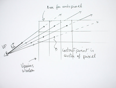
Direction vector for each pixel. Viewing window is divided into  areas
corresponding to each pixel in the image ( Illustration by Martin Bertrand)

It is useful to note that the create_unit_vector method returns our ray vector under a normalized form. This, once again, simplifies evaluating if results are appropriate as they are represented in world units.
Find if a collision occurs with the object
Now that we have established a normalized direction vector, the next step would be to verify if, for a particular ray, a collision occurs with a specific object. It is interesting to note that each type  of primitive object (polygon, sphere, cone, etc...) will have different formulas for calculating the intersection with the ray. 
The ray / sphere intersection is found by a combination of the ray's equation with the sphere's implicit equation we described earlier. We can then express this equation in terms of t. Since the complete details of this substitution can be found in Glassner's book (pp 36-37), we will just focus on the more general aspects of finding this t value and the interpretation of its value.
The substitution of the ray equation in the sphere's equation will yield, in terms of t, an equation of the form  A* t² + b*t + C = 0 a quadratic equation. The values of A, B and C, are easily found from elements we already possess like, the point of origin of the ray, the normalized vector, the center coordinates of the sphere. Once again, the detailed equations can be found in Glassner (pp 36-37).
Being a quadratic equation, t will have 2 potential values; But It is important to notice beforehand that if the discriminant of the quadratic equation is negative this ray misses the sphere entirely, and no further computation are necessary for this particular ray. If the discriminant is positive, then a collision has occurred. It is easy to implement a Boolean value that verifies this.
A positive discriminant will create two t values: These t values can either positive or negative. Only positive t values will be examined as they represent the distance in world units from the viewpoint to the intersection point. If 2 positive t values are found, only the smallest one should be considered to find the point of intersection as it is the one closest to viewpoint, therefore the only visible one if our object is not translucent. 
A quick summary of values:

• If discriminant is negative - no collision has occurred
• If t value negative, disregard, as intersection point with object is behind viewpoint
• Smallest positive t value is chosen to find intersection coordinate

If a collision occurs, find the world coordinates of the point of collision 

To find the actual coordinate of the point where the ray intersects is simple. It is inserted in our first ray equation. This is in fact also another useful method of the RayTracer class called get_intersection_point. It inputs a viewpoint (acting as ray origin) a unit direction vector, and the t value. It will return the coordinates of the point a distance of t from the origin.

public double[] get_intersection_point(double[] vp, double[] unit_vector, double t){

    double[] intersection = new double[3];

    for(int i = 0 ; i < 3 ; i++)

       intersection[i] = vp[i] + unit_vector[i] * t;

    return intersection;

}

This will yield the intersection's coordinate  for our particular ray and pixel. The next step would be calculate the light intensity at that particular point. To give our sphere the appearance of a 3-D volume, we will use the Phong shading algorithm at that point. We will describe this algorithm in the next section.

Implementation test

At this level, it would be useful to test if our ray / sphere intersection works properly. One simple way of doing so would be that if a ray sphere collision is detected, return a single fixed intensity value to the image buffer at the specified pixel. If the algorithm is successful, one should see a flat circle of uniform colour.

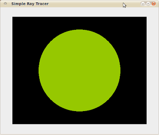
Successful Ray / Sphere intersection.
Here, a single colour value is given to all pixels.